SBiX

How SBiX works

F. Tria, E. Caglioti, V. Loreto and A. Pagnani
A stochastic local search algorithm for distance-based phylogeny reconstruction
Mol. Biol. Evol. (June, 2010).

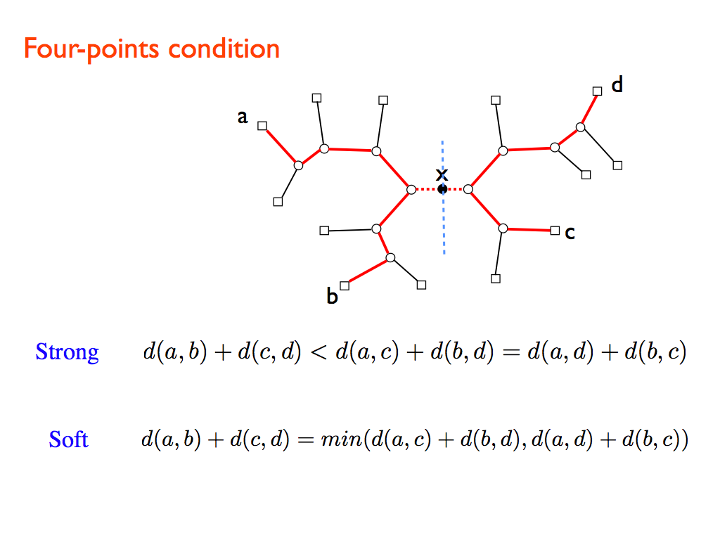
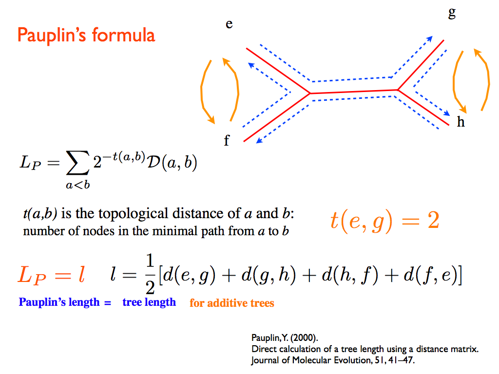
SBiX is a  distance-based algorithm for phylogenetic trees reconstruction based on a stochastic local search strategy in the space of all possible topologies of binary trees for a given set of taxa. It deeply exploits two fundamental properties of additive distances: the four-points condition and Pauplin’s formula.

The general structure of the SBiX algorithm is as follows:

1. start with a tree topology for the given set of  taxa;
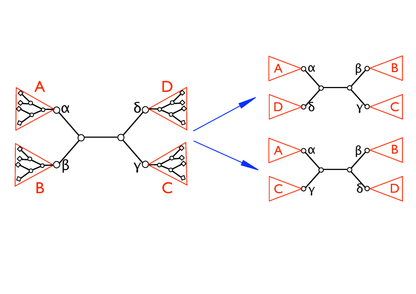
2. update the tree topology by local elementary rearrangements through Nearest Neighbor Interchange (see figure); one accepts the move with a MonteCarlo-like probability (see below);
3. repeat point 2 till convergence is reached;

Nearest Neighbor Interchange.

Simulated annealing and greedy strategy

1. In the simulated-annealing-like version of the algorithm we start with a random topology.  In the greedy version we search for a local minimum (which can eventually be the global one), so it is important to start with a meaningful topology.
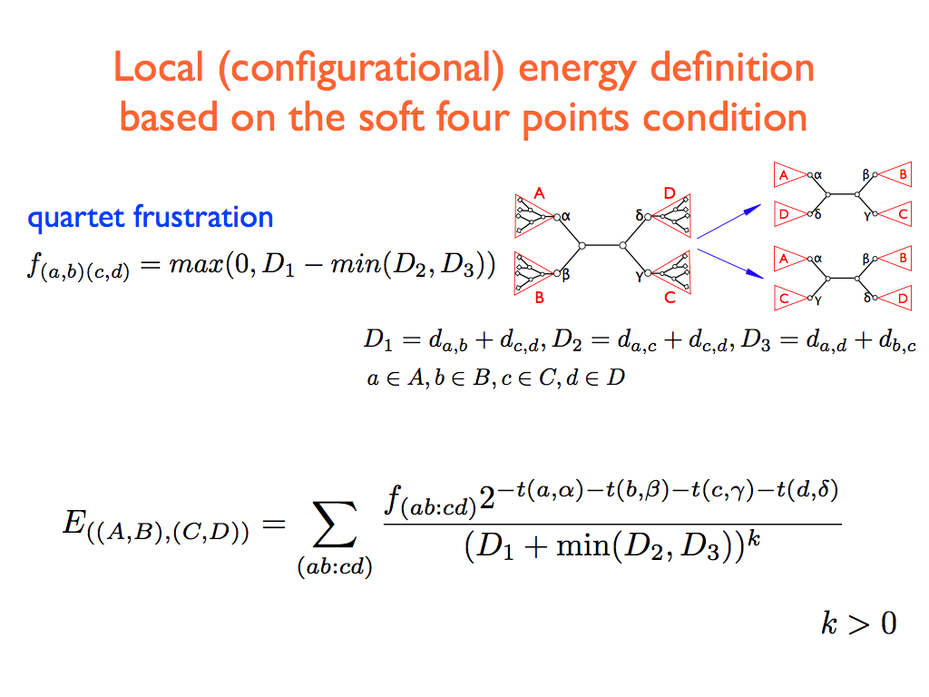
2. We sequentially consider all the internal edges of the present topology.  Each internal edge defines four subtrees (see the figure) say A,B,C,D, rooted respectively on the four internal nodes α,β,γ,δ.  Referring to fig. , let ((A,B),(C,D)) being the initial configuration.  We randomly choose one of the two possible local rewirings: (i) swap the pair B↔ D  getting the configuration ((A,D),(B,C)), (ii) swap the pair B ↔ C  getting the configuration ((A,C),(B,D)).  In the simulated-annealing version, the new configuration is accepted with probability one if  ΔE < 0 and a probability proportional to the statistical weight exp(-β sign(ΔE) if ΔE > 0, where β is an inverse temperature-like parameter that is set by a simulated annealing-like strategy (see point 3) and ΔE is the difference of the two configurations local costs: for case (i)    Δ E = E{((A,D),(B,C))} – E{((A,B),(C,D))} while for case (ii) ΔE = E{((A,C),(B,D))} – E{((A,B),(C,D))}.  In the greedy (or zero temperature) version, the new configuration is accepted if and only if Δ E < 0.
3. In the simulated-annealing version, we iterate point 2 starting with β=0 and increasing it at a constant rate at each sweep (we call a sweep an update of all the internal edges selected in a random permutation, so that each internal edge is selected once and only once,  with a different order, for each sweep) until convergence is reached, i.e., until the algorithm gets stuck in a fixed topology.  In the greedy version, we iterate point 2 until the algorithm gets stuck in a fixed topology.

Two versions available: SBiX and FastSBiX
We make here available two different strategies, namely SBiX and FastSBiX, the former in two different versions, namely a simulated-annealing-like and a greedy one. FastSBiX only features a greedy implementation, being based on the minimization of a local functional, which lacks its global counterpart. The SBiX algorithms features a computational complexity of O(N^4), where N is the number of taxa, although the greedy version is much more faster than the simulated annealing one. FastSBiX features a computational complexity of O(N^2 log(N)).

Dowload hereSBiX or FastSBiX.

After doing that extract the files from the .tar file, then just type “make” from a MS-DOS or Unix window inside the created directory.

GREEDY VERSION

SBiX and FastSBiX algorithms start from a given topology, and then improve that tree using Nearest Neigbor Interchanges (NNI) moves. The default initial topology is internally built using Fast Neighbor-Joining (FNJ) algortihm. Alternatively, the initial topology can be given as an input.

SBiX algorithms run from a MS-DOS or Unix window with the following options:

• -i specify the name of the input distance matrix in the PHYLIP format (see below for an example)
  
• -o desired name for the output topology, which will be given in the newick format
  
• -t if you want to start from a given topology, you must tipe “-t 1” (Default is t=0)
• -f if the option -t 1 is chosen, specify the name of the input tree, which has to be given in the newick format
• -h help menu
  

Example:

./sbix.exe (./fastsbix.exe)   -i  distmatrix -o outree

or

./sbix.exe (./fastsbix.exe)   -i  distmatrix -o outtree -t 1 -f inputtree

SIMULATED-ANNEALING-LIKE VERSION

This version of the algorithm is of course independent of the choice of the initial topology, so it is fair to use the defualt one. It is instead necessary to choose the cooling strategy. We call a sweep an update of all the edges of the tree and ß is the inverse-temperature-like parameter. It is necessary to select the number of sweeps n  and the interval Δß between two successive values of ß. Default values are setting as n=2 and Δß=0.0015 .

Dowload here SBiX Annealing .

After doing that extract the files from the .tar file, then just type “make” from a MS-DOS or Unix window inside the created directory.

SBiX_Annealing algorithm run from a MS-DOS or Unix window with the following options:

• -i specify the name of the input distance matrix in the PHYLIP format (see below for an example)
  
• -o desired name for the output topology, which will be given in the newick format
  
• -n number of sweeps with a fixed ß (Default is n=2)
• -b interval Δß between two successive values of ß (Default is Δß=0.0015)
• -h help menu
  

Example:

./sbix_ann.exe  -i  distmatrix -o outtree -n sweeps -b Δß

DISTANCE MATRIX FORMAT

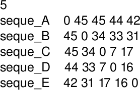
Distance matrices must be in the square PHYLIP format: they must have a single number on the first line that gives the number of taxa. Each subsequent line should contain the name of the taxon, followed by its distances to the other taxa. Note: taxon names should be less than 10 characters long.

Example:

To create a distance matrix one can use, for example,  DNADIST or PROTDIST of the PHYLIP libreries.

INITIAL TOPOLOGY AND OUTPUT TREE FORMAT

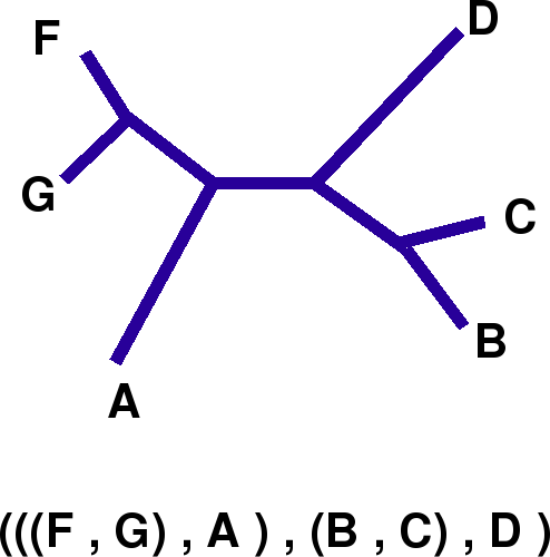
Input trees must be fully resolved, unrooted and written in the standard Newick Format. Output trees are also unrooted and given in the Newick format (it can be drawn using, for example DRAWGRAM or DRAWTREE of the PHYLIP libreries).

Example: a tree and its newick representation: